
Recently a customer who was contemplating switching their BI solution from an in-memory mode to a live SQL mode using Snowflake wanted to better understand the compute costs and user experience in the future state solution. Our reasoned but conservative cost estimates would be acceptable, if true, but this customer wanted to do realistic tests and see real performance data to confirm our assumptions and increase their confidence.
There was no specific question we were trying to answer, but instead we were trying to understand a fuzzy relationship between query performance, capacity, server size, and cost.
Here’s a simple overview of Snowflake compute cost, for background: a user consumes a credit by running a query and causing a node to come online. Once the node is active, others can also use capacity on it without incurring more credits. If that node gets too overloaded and busy, you can set rules for Snowflake to know when to justify burning another credit and adding another node to the cluster, ex., more than x concurrent queries, more than y seconds of queries queuing.

Transaction data does not support some important insights about what happened
We ran one user through realistic scenarios that generated dynamic SQL queries in Snowflake and query performance data we could analyze. The SNOWFLAKE.ACCOUNT_USAGE.QUERY_HISTORY table has one row per query with duration, start/end times, and other information, but nothing about concurrency, available capacity on the node, or the effect of concurrency on query run times.
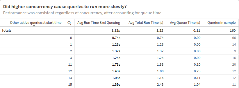
(Note: I did not detail it here, but we ran through similar tests with a larger Warehouse size and confirmed that query performance did not materially improve.)
I bet you have encountered similar situations. Some parallel use cases are analyzing Qlik session or reload data to understand concurrency, ex., what else was running that may have caused a file conflict and reload failure? A logically similar solution is using slowly changing dimensions with start/end dates or times to generate snapshots of employee or product data for headcount or product mix.
Converting Transactions to Periodic Snapshots unlocks trends and potentially hidden relationships
It’s difficult to detect trends without modeling the query transaction data differently. You can run one query simply enough to see what was happening at a single point in time, but it’s more work to understand what was happening across time to really tell the story of the data. Fortunately, there’s a data construct that enables this analysis called a Periodic Snapshot fact table.
A row in a periodic snapshot fact table summarizes many measurement events occurring over a standard period, such as a day, a week, or a month. The grain is the period, not the individual transaction.
In traditional Dimensional Modeling the rows for a period might be aggregated based on important dimensions, but in this case, we will keep the query rows as they are. This works well with Qlik’s associative model with modest data volumes, maintaining down-to-the-query detail. It’s also the type of challenge that makes me grateful for native transformation capabilities so you can solve your own data problem without leaving the app.

Raw materials needed to generate snapshots
Start/end dates or times on source rows
Our data has query start and end times, down to the fraction of a second. You may need to derive your own period end dates or times if they are not provided, based on sorting rows and using inter-record functions.
Overall start and end times of the analysis, i.e., first and last snapshots
We had 40 minutes of query activity for the testing period, from 1:00p to 1:40p.
Frequency of snapshots, AKA the period
For our data and use case, we chose snapshots every whole second. More common is daily snapshots. For older history, less frequent snapshots may be sufficient, like once a week or once a month.
Known limitation: transactions that start and end between two snapshots will not appear in our results, even though they still happened. Imagine if we captured snapshots every minute even though our queries generally run in less than one second: most queries would live their whole existences between snapshots and never appear in our results.

Generating snapshots with loops (slow, many loads)
The most common way I see snapshots generated in Qlik is using a loop. Each loop iteration generates one snapshot, autoconcatenated to the snapshot table.
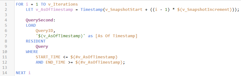
This code is admittedly simpler than what I will recommend, but you would have to add more logic if you wanted to generate a row for snapshots when no queries were running (important for our analysis).
The other downside is the reload time: it requires one load per snapshot, which could be hundreds or thousands, and the source table could be large. (The WHERE clause would also deoptimize QVD loads.) In my small sample set, this code took 7x as long to execute as what I advocate in the next section.
Generating snapshots with IntervalMatch (fast, few loads)
My preferred method for generating snapshots in Qlik is using IntervalMatch. This one load generates data for all instances of “As Of” dates or times between the start and end times in the table being loaded — the equivalent of a BETWEEN operator in SQL.

This code requires more discrete steps than the loop because of extra steps to resolve the synthetic key left behind by the IntervalMatch and the fact that Qlik is strict about what columns can be included in an IntervalMatch load. But a benefit of the IntervalMatch/LEFT JOIN load is that we will retain As Of Timestamp values when there were no queries running.
The other big upside is execution time. The IntervalMatch load is resource-intensive but will be finished running in a fraction of the time of the loops.
Ideas for extending the snapshot analysis
The QuerySecond snapshot table was an excellent start, but there were some deeper questions I wanted to answer.
- I created a Flag First Snapshot Active field for each query in the QuerySecond table for the first snapshot during which each query was active, to more easily analyze run times based on how busy the server was when a query started.
- I derived a Flag Has Concurrency Data field in the Query table so it would be easy to count how many queries were omitted from the snapshots entirely because they started and finished between successive snapshots.
- I created an As Of Timestamp table aggregating the active query count as of each second to make it easier to do analysis using the number of active queries as a dimension.
These data elements were used to build the screenshots in this post and can also be found in the linked, complete solution: Snapshots.zip (includes QVF and sample data)
Bonus tip: Remove source rows to speed up snapshot generation
Whichever approach you take, here is one way to speed up generating snapshots and consume fewer resources in the process: remove as many rows as you can from the resident source table before generating snapshots with it. Here are some candidates for removal:
- Rows with zero values for all metrics (or, e.g., for headcount, exclude rows with intervals during which the employee was inactive)
- Rows with an end date before your first snapshot or a start date after your last snapshot
- Rows where the start and end dates do not cross over any snapshot intervals, i.e., they will never be part of any snapshot